DO NOT COPY FROM CHEGG OR COURSEHERO…MY PROFESSOR WILL KNOW AND I WILL GET A ZERO

Week 7 Assignment

Question 1

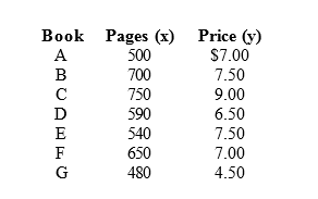
Assume you have noted the following prices for paperback books and the number of pages that each book contains.
Develop a least-squares estimated regression line.

1. Go to Excel. Create a scatter diagram for the data. Include the trendline (regression line). Make sure from Week 1 you know what a trendline is. It is NOT simply connecting the dots.
2. Once the scatter diagram is created, right-click on the trendline itself in the graph. Use the “format trendline” from the menu to show the equation of the trendline and the r squared value on the graph itself.
3. You will now create a table of values like the ones on page 536 and 537 for this data. The table will include:
   1. Pages (x) – at the bottom of this column, find the mean of the x values. You will need this later.
   2. Price (y) – at the bottom of this column, find the mean of the y values. You will need this later.
   3. Predicted value – List the equation of the trendline (regression line) from your scatter plot. Plug in each value of x into the equation and solve it. This is your
   4. Error – take each given y value minus the predicted y value – column 2 minus column 3.
   5. Squared error – square each value in the error column.At the bottom of the column, add up all the values. This is your SSE. Label it. You will need it later.
   6. Deviation – take each y value minus the mean y value that you calculated earlier. (This is why you put the mean value of y under your second column).
   7. Squared deviation. Square each value in the deviation column. Add up your squared deviations at the bottom of the column. This is your SST. Label it. You will need it later.
   8. Go to page 538 and find the formula that shows the relationship between the SST, SSR, and SSE. You calculated SST and SSE. Solve for SSR. Label it.
4. Compute the coefficient of determination and explain its meaning. This is found on page 539. Make sure that your calculation matches what is in your graph for r squared. If it does not match, go back and find the error.
5. Compute the correlation coefficient between the price and the number of pages.(p. 540)
6. Test to see if x and y are related. Use α = 0.10. You will be using the t-test formula around page 546,
   1. What are the degrees of freedom for this test?
   2. Calculate s – the Standard Error of the Estimate using your SSE.
   3. Go back to the table to add two more columns. The first one is where you will subtract the mean of the x values from each x value.
   4. The second column you will create will contain the square of the values you just created – square the difference between each x value and the mean for the x values. Add this column up for a total of these squared values.
   5. Go to page 547 and calculate the estimated standard deviation of sb1. You will need the standard error of the estimate (s) that you calculated and the sum of the squared differences between x and the mean of x.
   6. The t value calculation involves the slope from the regression line (trendline) from your graph and the sb1 that you just calculated. Find the t test statistic.
   7. Use the yellow box at the bottom of p. 547 to determine if your t value indicates that the null hypothesis should be rejected or if it should fail to be rejected. Explain why you rejected/failed to reject it.

Question 2

The following data represent a company’s yearly sales volume and its advertising expenditure over a period of 8 years.

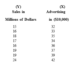
1. Develop a scatter diagram of sales versus advertising and explain what it shows regarding the relationship between sales and advertising.
2. Use the method of least squares to compute an estimated regression line between sales and advertising OR just show it on the graph along with your r-squared value..
3. If the company’s advertising expenditure is $400,000, what are the predicted sales? Give the answer in dollars. (This is found using algebra and the equation of the trendline / regression line – make sure to watch your units)
4. What does the slope of the estimated regression line indicate?

Project Week 7

For these project assignments throughout the course you will need to reference the data in the ROI Excel spreadheet. Download it here.

Using the ROI data set:

The step by step directions from the assignment may also be applied here. They may be helpful.

For each of the two majors:

1. Draw the scatter diagram of Y = ‘Annual % ROI’ against X = ‘Cost’. Include the trendline (regression line) and the r-squared value (coefficient of determination).
2. Obtain b0 and b1 of the regression equation defined as y ̂ = b0 + b1X (y intercept and slope).
3. Calculate the estimated ‘Annual % ROI’ when the ‘Cost’ (X) is $160,000. (algebra using the equation of the line)
   • H0: β1 = 0
   • Ha: β1 ≠ 0
   • Write a paragraph or more on any observations you make about the regression estimates, coefficient of determination, the plots, and the results of your hypothesis tests. Please note the plural nature – paragraph or MORE, hypothesis testS – there is a focus on the comprehensive nature of this final part of the project. One way to set this part of the project up is to first talk about each test – what is it, what does it test for? Then show your work and discuss the outcome. Repeat this for each test. Summarize findings at the end.

Test the hypothesis: You will need to show work for the tests you are performing – t-tests, F tests…see the end of chapter 12 to make sure you are doing a comprehensive analysis.